Generate a binary population by hand
The process to generate a synthetic binary population, is similar to the
process to evolve a single/multiple binaries by hand: first generate an
initial population, then evolve it with the Evolve class.
An initialized binary population consists of a collection of binary systems with assigned primary and secondary masses, orbital periods, eccentricities, metallicities, and star formation histories. These parameters are randomly sampled from observationally motivated distribution functions.
In COSMIC, the initial sample is done through an initial binary sampler which works
with the InitialBinaryTable class. There are two samplers available:
1. independent : initialize binaries with independent parameter distributions for the primary mass, mass ratio, eccentricity, separation, and binary fraction
2. multidim : initialize binaries with multidimensional parameter distributions according to Moe & Di Stefano 2017
We consider both cases below.
independent
First import the InitialBinaryTable class and the independent sampler
In [1]: from cosmic.sample.initialbinarytable import InitialBinaryTable

In [2]: from cosmic.sample.sampler import independent
The independent sampler contains multiple models for each binary parameter. You can access the available models using the independent sampler help call:
In [3]: help(independent.get_independent_sampler)
Help on function get_independent_sampler in module cosmic.sample.sampler.independent:

get_independent_sampler(final_kstar1, final_kstar2, primary_model, ecc_model, porb_model, SF_start, SF_duration, binfrac_model, met, size=None, total_mass=inf, sampling_target='size', trim_extra_samples=False, q_power_law=0, **kwargs)
    Generates an initial binary sample according to user specified models

    Parameters
    ----------
    final_kstar1 : `int or list`
        Int or list of final kstar1

    final_kstar2 : `int or list`
        Int or list of final kstar2

    primary_model : `str`
        Model to sample primary mass; choices include: kroupa93, kroupa01, salpeter55, custom
        if 'custom' is selected, must also pass arguemts:
        alphas : `array`
            list of power law indicies
        mcuts : `array`
            breaks in the power laws.
        e.g. alphas=[-1.3,-2.3,-2.3],mcuts=[0.08,0.5,1.0,150.] reproduces standard Kroupa2001 IMF

    ecc_model : `str`
        Model to sample eccentricity; choices include: thermal, uniform, sana12

    porb_model : `str` or `dict`
        Model to sample orbital period; choices include: log_uniform, sana12, raghavan10, moe19
        or a custom power law distribution defined with a dictionary with keys "min", "max", and "slope"
        (e.g. {"min": 0.15, "max": 0.55, "slope": -0.55}) would reproduce the Sana+2012 distribution

    qmin : `float`
        kwarg which sets the minimum mass ratio for sampling the secondary
        where the mass ratio distribution is flat in q
        if q > 0, qmin sets the minimum mass ratio
        q = -1, this limits the minimum mass ratio to be set such that
        the pre-MS lifetime of the secondary is not longer than the full
        lifetime of the primary if it were to evolve as a single star

    m_max : `float`
        kwarg which sets the maximum primary and secondary mass for sampling
        NOTE: this value changes the range of the IMF and should *not* be used
            as a means of selecting certain kstar types!

    m1_min : `float`
        kwarg which sets the minimum primary mass for sampling
        NOTE: this value changes the range of the IMF and should *not* be used
            as a means of selecting certain kstar types!

    m2_min : `float`
        kwarg which sets the minimum secondary mass for sampling
        the secondary as uniform in mass_2 between m2_min and mass_1

    msort : `float`
        Stars with M>msort can have different pairing and sampling of companions

    qmin_msort : `float`
        Same as qmin for M>msort

    m2_min_msort : `float`
        Same as m2_min for M>msort

    SF_start : `float`
        Time in the past when star formation initiates in Myr

    SF_duration : `float`
        Duration of constant star formation beginning from SF_Start in Myr

    binfrac_model : `str or float`
        Model for binary fraction; choices include: vanHaaften, offner22, or a fraction where 1.0 is 100% binaries

    binfrac_model_msort : `str or float`
        Same as binfrac_model for M>msort

    met : `float`
        Sets the metallicity of the binary population where solar metallicity is zsun

    size : `int`
        Size of the population to sample

    total_mass : `float`
        Total mass to use as a target for sampling

    sampling_target : `str`
        Which type of target to use for sampling (either "size" or "total_mass"), by default "size".
        Note that `total_mass` must not be None when `sampling_target=="total_mass"`.

    trim_extra_samples : `str`
        Whether to trim the sampled population so that the total mass sampled is as close as possible to
        `total_mass`. Ignored when `sampling_target==size`.
        Note that given the discrete mass of stars, this could mean your sample is off by 300
        solar masses in the worst case scenario (of a 150+150 binary being sampled). In reality the majority
        of cases track the target total mass to within a solar mass.

    zsun : `float`
        optional kwarg for setting effective radii, default is 0.02

    q_power_law : `float`
        Exponent for the mass ratio distribution power law, default is 0 (flat in q). Note that
        q_power_law cannot be exactly -1, as this would result in a divergent distribution.


    Returns
    -------
    InitialBinaryTable : `pandas.DataFrame`
        DataFrame in the format of the InitialBinaryTable

    mass_singles : `float`
        Total mass in single stars needed to generate population

    mass_binaries : `float`
        Total mass in binaries needed to generate population

    n_singles : `int`
        Number of single stars needed to generate a population

    n_binaries : `int`
        Number of binaries needed to generate a population
Targetting specific final kstar types
The final_kstar1 and final_kstar2 parameters are lists that contain the kstar types
that you would like the final population to contain.
The final kstar is the final state of the binary system we are interested in and is based on the BSE kstar naming convention, see Evolutionary State of the Star for more information.
Thus, if you want to generate a population containing double white dwarfs with CO and ONe WD primaries and He-WD secondaries, the final kstar inputs would be:
In [4]: final_kstar1 = [11, 12]

In [5]: final_kstar2 = [10]
Since we are interested in binaries, we only retain the binary systems that are likely to produce the user specified final kstar types. However, we also keep track of the total mass of the single and binary stars as well as the number of binary and single stars so that we can scale our results to larger populations. If you don’t want to filter the binaries, you can supply final kstars as
In [6]: final_kstars = np.linspace(0, 14, 15)

In [7]: InitialBinaries, mass_singles, mass_binaries, n_singles, n_binaries = InitialBinaryTable.sampler('independent', final_kstars, final_kstars, binfrac_model=0.5, primary_model='kroupa01', ecc_model='sana12', porb_model='sana12', qmin=-1, m2_min=0.08, SF_start=13700.0, SF_duration=0.0, met=0.02, size=10000)
Additionally if you are interested in single stars then you can specify keep_singles=True.
Understanding parameter sampling models
Similar to the help for the sampler, the different models that can be used for each parameter to be sampled can be accessed by the help function for the argument. The syntax for each parameter sample is always: sample_`parameter`. See the example for the star formation history (SFH) below:
In [8]: help(independent.Sample.sample_SFH)
Help on function sample_SFH in module cosmic.sample.sampler.independent:

sample_SFH(self, SF_start=13700.0, SF_duration=0.0, met=0.02, size=None)
    Sample an evolution time for each binary based on a user-specified
    time at the start of star formation and the duration of star formation.
    The default is a burst of star formation 13,700 Myr in the past.

    Parameters
    ----------
    SF_start : float
        Time in the past when star formation initiates in Myr
    SF_duration : float
        Duration of constant star formation beginning from SF_Start in Myr
    met : float
        metallicity of the population [Z_sun = 0.02]
        Default: 0.02
    size : int, optional
        number of evolution times to sample
        NOTE: this is set in cosmic-pop call as Nstep

    Returns
    -------
    tphys : array
        array of evolution times of size=size
    metallicity : array
        array of metallicities
Stopping conditions for sampling
In addition to telling COSMIC how to sample, you also need to tell it how much to sample. You can
do this in one of two ways: (1) by specifying the number of binaries to sample, or (2) by specifying the total mass of singles and binaries to sample. Let’s look at both of these in more detail.
Number of binaries
Using the final kstar inputs we mentioned above, the initial binary population can be sampled based on the desired number of binaries (10000 in this case) as follows
In [9]: InitialBinaries, mass_singles, mass_binaries, n_singles, n_binaries = InitialBinaryTable.sampler('independent', final_kstar1, final_kstar2, binfrac_model=0.5, primary_model='kroupa01', ecc_model='sana12', porb_model='sana12', qmin=-1, m2_min=0.08, SF_start=13700.0, SF_duration=0.0, met=0.02, size=10000)

In [10]: print(InitialBinaries)
       kstar_1  kstar_2     mass_1  ...  bhspin_2  tphys  binfrac
0          1.0      1.0   3.853043  ...       0.0    0.0      0.5
1          1.0      0.0   0.977576  ...       0.0    0.0      0.5
2          1.0      1.0  14.509648  ...       0.0    0.0      0.5
3          1.0      1.0   0.880338  ...       0.0    0.0      0.5
4          1.0      1.0   1.808589  ...       0.0    0.0      0.5
...        ...      ...        ...  ...       ...    ...      ...
10409      1.0      1.0  18.345183  ...       0.0    0.0      0.5
10410      1.0      0.0   0.918056  ...       0.0    0.0      0.5
10411      1.0      1.0   0.984430  ...       0.0    0.0      0.5
10412      1.0      0.0   2.014796  ...       0.0    0.0      0.5
10413      1.0      1.0   1.480655  ...       0.0    0.0      0.5

[10414 rows x 38 columns]
Note
The length of the initial binary data set, InitialBinaries, does not always match
the size parameter provided to sampler().
This is because of the various cuts that the sampler makes to the population (e.g. the binary fraction,
which is either a fraction between 0 and 1 or mass dependent following the
prescription in van Haaften+2013.) specified by the user.
Total mass sampled
Alternatively, we could do the same thing but now instead set our sampling_target to be the total mass and aim for 15000 solar masses. This is done by setting sampling_target="total_mass" and total_mass=15000.
In [11]: InitialBinaries, mass_singles, mass_binaries, n_singles, n_binaries = InitialBinaryTable.sampler('independent', final_kstar1, final_kstar2, binfrac_model=0.5, primary_model='kroupa01', ecc_model='sana12', porb_model='sana12', qmin=-1, m2_min=0.08, SF_start=13700.0, SF_duration=0.0, met=0.02, sampling_target="total_mass", total_mass=15000)

In [12]: print(InitialBinaries)
      kstar_1  kstar_2    mass_1    mass_2  ...  bhspin_1  bhspin_2  tphys  binfrac
0         1.0      1.0  3.333541  0.843308  ...       0.0       0.0    0.0      0.5
1         1.0      1.0  1.259961  0.769420  ...       0.0       0.0    0.0      0.5
2         1.0      1.0  1.644375  1.454379  ...       0.0       0.0    0.0      0.5
3         1.0      1.0  1.003911  0.864505  ...       0.0       0.0    0.0      0.5
4         1.0      1.0  3.038599  2.729126  ...       0.0       0.0    0.0      0.5
...       ...      ...       ...       ...  ...       ...       ...    ...      ...
1365      1.0      0.0  2.659504  0.531773  ...       0.0       0.0    0.0      0.5
1366      1.0      0.0  0.882433  0.677457  ...       0.0       0.0    0.0      0.5
1367      1.0      1.0  2.934133  2.025925  ...       0.0       0.0    0.0      0.5
1368      1.0      1.0  1.907866  1.146731  ...       0.0       0.0    0.0      0.5
1369      1.0      0.0  0.971765  0.630025  ...       0.0       0.0    0.0      0.5

[1370 rows x 38 columns]
And we can check what the total sampled mass was by looking at the sum of the mass_singles and mass_binaries variables
In [13]: print(mass_singles + mass_binaries)
22865.40198110109
Tip
If you’d like to avoid your sample overshooting your desired total_mass and instead get as close to this value as possible,
you can set trim_extra_samples=True. This will trim the sample to get a total mass as close as possible to your target.
In many cases, this will be within a solar mass, but could be as large as twice the maximum stellar mass (for the very rare case that
the final binary drawn is the most massive primary with an equal mass ratio).
Mass dependent binary fractions and mass pairings
If you want to have separate binary fractions and mass pairings for low and high mass stars, you can by supplying the msort kwarg to the sampler. This sets the mass above which an alternative mass pairing (specified by kwargs qmin_msort and m2_min_msort) and binary fraction model (specified by kwarg binfrac_model_msort) are used. This is handy if you want, for example, a higher binary fraction and more equal mass pairings for high mass stars.
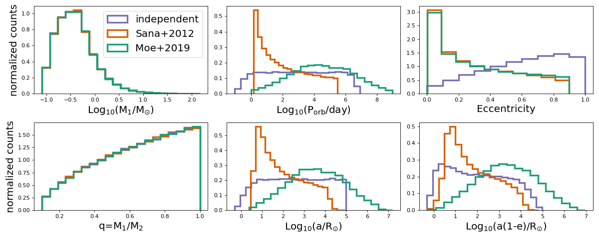
Below we show the effect of different assumptions for the independent initial sampler. The standard assumptions are shown in purple, the assumptions of Sana et al. 2012 are shown in orange, and the assumptions of Moe et al. 2019 are shown in green.
(Source code, png, hires.png, pdf)
multidim
COSMIC implements multidimensionally distributed initial binaries according to Moe & Di Stefano 2017. The python code used in COSMIC to create this sample was written by Mads Sorenson, and is based on the IDL codes written to accompany Moe & Di Stefano 2017.
The multidimensional initial binary data is sampled in COSMIC as follows:
In [14]: from cosmic.sample.initialbinarytable import InitialBinaryTable

In [15]: from cosmic.sample.sampler import multidim
To see the arguments necessary to call the multidimensional sampler use the help function:
In [16]: help(multidim.get_multidim_sampler)
Help on function get_multidim_sampler in module cosmic.sample.sampler.multidim:

get_multidim_sampler(final_kstar1, final_kstar2, rand_seed, nproc, SF_start, SF_duration, met, size, **kwargs)
    adapted version of Maxwell Moe's IDL code that generates a population of single and binary stars

    Below is the adapted version of Maxwell Moe's IDL code
    that generates a population of single and binary stars
    based on the paper Mind your P's and Q's
    By Maxwell Moe and Rosanne Di Stefano

    The python code has been adopted by Mads Sørensen

    Version history:
    V. 0.1; 2017/02/03
    By Mads Sørensen
    - This is a pure adaption from IDL to Python.
    - The function idl_tabulate is similar to
    the IDL function int_tabulated except, this function seems to be slightly
    more exact in its solution.
    Therefore, relative to the IDL code, there are small numerical differences.

    Comments below beginning with ; is the original nodes by Maxwell Moe.
    Please read these careful for understanding the script.
    ; NOTE - This version produces only the statistical distributions of
    ;        single stars, binaries, and inner binaries in hierarchical triples.
    ;        Outer tertiaries in hierarchical triples are NOT generated.
    ;        Moreover, given a set of companions, all with period P to
    ;        primary mass M1, this version currently uses an approximation to
    ;        determine the fraction of those companions that are inner binaries
    ;        vs. outer triples. Nevertheless, this approximation reproduces
    ;        the overall multiplicity statistics.
    ; Step 1 - Tabulate probably density functions of periods,
    ;          mass ratios, and eccentricities based on
    ;          analytic fits to corrected binary star populations.
    ; Step 2 - Implement Monte Carlo method to generate stellar
    ;          population from those density functions.

    Parameters
    ----------
    final_kstar1 : `list` or `int`
        Int or list of final kstar1

    final_kstar2 : `list` or `int`
        Int or list of final kstar2

    rand_seed : `int`
        Int to seed random number generator

    nproc : `int`
        Number of processors to use to generate population

    SF_start : `float`
            Time in the past when star formation initiates in Myr

    SF_duration : `float`
            Duration of constant star formation beginning from SF_Start in Myr

    met : `float`
        Sets the metallicity of the binary population where solar metallicity is 0.02

    size : `int`
        Size of the population to sample

    **porb_lo : `float`
        Lower limit in days for the orbital period distribution

    **porb_hi: `float`
        Upper limit in days for the orbital period distribution

    Returns
    -------
    InitialBinaryTable : `pandas.DataFrame`
        DataFrame in the format of the InitialBinaryTable

    mass_singles : `float`
        Total mass in single stars needed to generate population

    mass_binaries : `float`
        Total mass in binaries needed to generate population

    n_singles : `int`
        Number of single stars needed to generate a population

    n_binaries : `int`
        Number of binaries needed to generate a population
The random seed is used to reproduce your initial sample, since there are several stochastic processes involved in the muldimensional sample. As in the independent sampler, the final_kstar1 and final_kstar2 inputs are lists containing the kstar types that the evolved population should contain.
The multidimensional sample is generated as follows:
In [17]: InitialBinaries, mass_singles, mass_binaries, n_singles, n_binaries = InitialBinaryTable.sampler('multidim', final_kstar1=[11], final_kstar2=[11], rand_seed=2, nproc=1, SF_start=13700.0, SF_duration=0.0, met=0.02, size=10)

In [18]: print(InitialBinaries)
   kstar_1  kstar_2     mass_1    mass_2  ...  bhspin_1  bhspin_2  tphys   binfrac
0      1.0      1.0   6.180111  0.811538  ...       0.0       0.0    0.0  0.806628
1      1.0      1.0   1.512334  0.941730  ...       0.0       0.0    0.0  0.442176
2      1.0      1.0   1.118342  1.060351  ...       0.0       0.0    0.0  0.411491
3      1.0      1.0   1.282262  1.276681  ...       0.0       0.0    0.0  0.421378
4      1.0      1.0   3.123983  1.071289  ...       0.0       0.0    0.0  0.576703
5      1.0      1.0   3.051238  1.283223  ...       0.0       0.0    0.0  0.568435
6      1.0      1.0  10.380407  9.784358  ...       0.0       0.0    0.0  0.857319
7      1.0      1.0   4.537656  2.647862  ...       0.0       0.0    0.0  0.680490
8      1.0      1.0   1.928006  1.178359  ...       0.0       0.0    0.0  0.478645
9      1.0      1.0   1.565922  1.287431  ...       0.0       0.0    0.0  0.447819

[10 rows x 38 columns]
Note
NOTE that in the multidimensional case, the binary fraction is a parameter in the sample. This results in the size of the initial binary data matching the size provided to the sampler. As in the independent sampling case, we keep track of the total sampled mass of singles and binaries as well as the total number of single and binary stars to scale thesimulated population to astrophysical populations.
Evolving an initial binary population
As in Using COSMIC to evolve binaries, once an initial binary population is sampled, it is evolved using the Evolve class. Note that the same process used in Using COSMIC to evolve binaries applies here as well: the BSEDict must be supplied, but only need be resupplied if the flags in the dictionary change.
The syntax for the Evolve class is as follows:
In [19]: from cosmic.evolve import Evolve

In [20]: BSEDict = {'xi': 1.0, 'bhflag': 1, 'neta': 0.5, 'windflag': 3, 'wdflag': 1, 'alpha1': 1.0, 'pts1': 0.001, 'pts3': 0.02, 'pts2': 0.01, 'epsnov': 0.001, 'hewind': 0.5, 'ck': 1000, 'bwind': 0.0, 'lambdaf': 0.0, 'mxns': 3.0, 'beta': -1.0, 'tflag': 1, 'acc2': 1.5, 'grflag' : 1, 'remnantflag': 4, 'ceflag': 0, 'eddfac': 1.0, 'ifflag': 0, 'bconst': 3000, 'sigma': 265.0, 'gamma': -2.0, 'pisn': 45.0, 'natal_kick_array' : [[-100.0,-100.0,-100.0,-100.0,0.0], [-100.0,-100.0,-100.0,-100.0,0.0]], 'bhsigmafrac' : 1.0, 'polar_kick_angle' : 90, 'qcrit_array' : [0.0,0.0,0.0,0.0,0.0,0.0,0.0,0.0,0.0,0.0,0.0,0.0,0.0,0.0,0.0,0.0], 'cekickflag' : 2, 'cehestarflag' : 0, 'cemergeflag' : 0, 'ecsn' : 2.25, 'ecsn_mlow' : 1.6, 'aic' : 1, 'ussn' : 0, 'sigmadiv' :-20.0, 'qcflag' : 1, 'eddlimflag' : 0, 'fprimc_array' : [2.0/21.0,2.0/21.0,2.0/21.0,2.0/21.0,2.0/21.0,2.0/21.0,2.0/21.0,2.0/21.0,2.0/21.0,2.0/21.0,2.0/21.0,2.0/21.0,2.0/21.0,2.0/21.0,2.0/21.0,2.0/21.0], 'bhspinflag' : 0, 'bhspinmag' : 0.0, 'rejuv_fac' : 1.0, 'rejuvflag' : 0, 'htpmb' : 1, 'ST_cr' : 1, 'ST_tide' : 1, 'bdecayfac' : 1, 'rembar_massloss' : 0.5, 'kickflag' : 0, 'zsun' : 0.019, 'bhms_coll_flag' : 0, 'don_lim' : -1, 'acc_lim' : -1, 'rtmsflag' : 0, 'wd_mass_lim' : 1}

In [21]: bpp, bcm, initC, kick_info  = Evolve.evolve(initialbinarytable=InitialBinaries, BSEDict=BSEDict)

In [22]: print(bcm.iloc[:10])
     tphys  kstar_1   mass0_1    mass_1  ...  SN_2  bin_state  merger_type  bin_num
0      0.0      1.0  6.180111  6.180111  ...   0.0          0         -001        0
0  13700.0     11.0  1.156558  1.156558  ...   0.0          0         -001        0
1      0.0      1.0  1.512334  1.512334  ...   0.0          0         -001        1
1  13700.0     11.0  0.573866  0.573866  ...   0.0          0         -001        1
2      0.0      1.0  1.118342  1.118342  ...   0.0          0         -001        2
2  13700.0     11.0  0.573694  0.573694  ...   0.0          1         0301        2
3      0.0      1.0  1.282262  1.282262  ...   0.0          0         -001        3
3  13700.0     11.0  0.545384  0.545384  ...   0.0          0         -001        3
4      0.0      1.0  3.123983  3.123983  ...   0.0          0         -001        4
4  13700.0     11.0  0.756901  0.756903  ...   0.0          0         -001        4

[10 rows x 39 columns]

In [23]: print(bpp)
           tphys    mass_1    mass_2  ...  bhspin_1  bhspin_2  bin_num
0       0.000000  6.180111  0.811538  ...       0.0       0.0        0
0      64.185978  6.156144  0.811538  ...       0.0       0.0        0
0      64.415045  6.155656  0.811538  ...       0.0       0.0        0
0      64.512065  6.154358  0.811538  ...       0.0       0.0        0
0      72.950683  6.058549  0.811539  ...       0.0       0.0        0
..           ...       ...       ...  ...       ...       ...      ...
9    4966.919572  0.518098  0.266712  ...       0.0       0.0        9
9    4966.919572  0.518098  0.266712  ...       0.0       0.0        9
9    7329.998839  0.518098  0.266712  ...       0.0       0.0        9
9    7330.009792  0.000000  0.180555  ...       0.0       0.0        9
9   13700.000000  0.000000  0.180555  ...       0.0       0.0        9

[138 rows x 44 columns]
ClusterMonteCarlo
New in COSMIC 3.4, you can now use COSMIC to sample initial conditions that can be used in the simulation of a Globular Cluster (GC), using the ClusterMonteCarlo (CMC) software package. To create these initial conditions, and save them in a format readable by CMC, you can do the following.
In [24]: from cosmic.sample.initialcmctable import InitialCMCTable

In [25]: from cosmic.sample.sampler import cmc
To see the arguments necessary to call the CMC sampler use the help function:
In [26]: help(cmc.get_cmc_sampler)
Help on function get_cmc_sampler in module cosmic.sample.sampler.cmc:

get_cmc_sampler(cluster_profile, primary_model, ecc_model, porb_model, binfrac_model, met, size, **kwargs)
    Generates an initial cluster sample according to user specified models

    Parameters
    ----------
    cluster_profile : `str`
        Model to use for the cluster profile (i.e. sampling of the placement of objects in the cluster and their velocity within the cluster)
        Options include:
        'plummer' : Standard Plummer sphere.
            Additional parameters:
            'r_max' : `float`
                the maximum radius (in virial radii) to sample the clsuter
        'elson' : EFF 1987 profile.  Generalization of Plummer that better fits young massive clusters
            Additional parameters:
            'gamma' : `float`
                steepness paramter for Elson profile; note that gamma=4 is same is Plummer
            'r_max' : `float`
                the maximum radius (in virial radii) to sample the clsuter
        'king' : King profile
            'w_0' : `float`
                King concentration parameter
            'r_max' : `float`
                the maximum radius (in virial radii) to sample the clsuter

    primary_model : `str`
        Model to sample primary mass; choices include: kroupa93, kroupa01, salpeter55, custom
        if 'custom' is selected, must also pass arguemts:
        alphas : `array`
            list of power law indicies
        mcuts : `array`
            breaks in the power laws.
        e.g. alphas=[-1.3,-2.3,-2.3],mcuts=[0.08,0.5,1.0,150.] reproduces standard Kroupa2001 IMF

    ecc_model : `str`
        Model to sample eccentricity; choices include: thermal, uniform, sana12

    porb_model : `str`
        Model to sample orbital period; choices include: log_uniform, sana12

    msort : `float`
        Stars with M>msort can have different pairing and sampling of companions

    pair : `float`
        Sets the pairing of stars M>msort only with stars with M>msort

    binfrac_model : `str or float`
        Model for binary fraction; choices include: vanHaaften, offner22, or a fraction where 1.0 is 100% binaries

    binfrac_model_msort : `str or float`
        Same as binfrac_model for M>msort

    qmin : `float`
        kwarg which sets the minimum mass ratio for sampling the secondary
        where the mass ratio distribution is flat in q
        if q > 0, qmin sets the minimum mass ratio
        q = -1, this limits the minimum mass ratio to be set such that
        the pre-MS lifetime of the secondary is not longer than the full
        lifetime of the primary if it were to evolve as a single star

    m2_min : `float`
        kwarg which sets the minimum secondary mass for sampling
        the secondary as uniform in mass_2 between m2_min and mass_1

    qmin_msort : `float`
        Same as qmin for M>msort; only applies if qmin is supplied

    met : `float`
        Sets the metallicity of the binary population where solar metallicity is zsun

    size : `int`
        Size of the population to sample

    zsun : `float`
        optional kwarg for setting effective radii, default is 0.02

    Optional Parameters
    -------------------
    virial_radius : `float`
        the initial virial radius of the cluster, in parsecs
        Default -- 1 pc

    tidal_radius : `float`
        the initial tidal radius of the cluster, in units of the virial_radius
        Default -- 1e6 rvir

    central_bh : `float`
        Put a central massive black hole in the cluster
        Default -- 0 MSUN

    scale_with_central_bh : `bool`
        If True, then the potential from the central_bh is included when scaling the radii.
        Default -- False

    seed : `float`
        seed to the random number generator, for reproducability

    Returns
    -------
    Singles: `pandas.DataFrame`
        DataFrame of Single objects in the format of the InitialCMCTable

    Binaries: `pandas.DataFrame`
        DataFrame of Single objects in the format of the InitialCMCTable
In [27]: from cosmic.sample import InitialCMCTable

In [28]: Singles, Binaries = InitialCMCTable.sampler('cmc', binfrac_model=0.2, primary_model='kroupa01', ecc_model='sana12', porb_model='sana12', qmin=-1.0, cluster_profile='plummer', met=0.014, size=40000, params='../examples/Params.ini', gamma=4, r_max=100)

In [29]: InitialCMCTable.write(Singles, Binaries, filename="input.hdf5")

In [30]: InitialCMCTable.write(Singles, Binaries, filename="input.fits")