Generate a binary population by hand
The process to generate a synthetic binary population, is similar to the process to evolve a single/multiple binaries by hand: first generate an initial population, then evolve it with the Evolve class.
An initialized binary population consists of a collection of binary systems with assigned primary and secondary masses, orbital periods, eccentricities, metallicities, and star formation histories. These parameters are randomly sampled from observationally motivated distribution functions.
In COSMIC, the initial sample is done through an initial binary sampler which works with the InitialBinaryTable class. There are two samplers available:
1. independent : initialize binaries with independent parameter distributions for the primary mass, mass ratio, eccentricity, separation, and binary fraction
2. multidim : initialize binaries with multidimensional parameter distributions according to Moe & Di Stefano 2017
We consider both cases below.
independent
First import the InitialBinaryTable class and the independent sampler
In [1]: from cosmic.sample.initialbinarytable import InitialBinaryTable

In [2]: from cosmic.sample.sampler import independent
The independent sampler contains multiple models for each binary parameter. You can access the available models using the independent sampler help call:
In [3]: help(independent.get_independent_sampler)
Help on function get_independent_sampler in module cosmic.sample.sampler.independent:

get_independent_sampler(final_kstar1, final_kstar2, primary_model, ecc_model, porb_model, SF_start, SF_duration, binfrac_model, met, size, **kwargs)
    Generates an initial binary sample according to user specified models

    Parameters
    ----------
    final_kstar1 : `int or list`
        Int or list of final kstar1

    final_kstar2 : `int or list`
        Int or list of final kstar2

    primary_model : `str`
        Model to sample primary mass; choices include: kroupa93, kroupa01, salpeter55

    ecc_model : `str`
        Model to sample eccentricity; choices include: thermal, uniform, sana12

    porb_model : `str`
        Model to sample orbital period; choices include: log_uniform, sana12

    SF_start : `float`
            Time in the past when star formation initiates in Myr

    SF_duration : `float`
            Duration of constant star formation beginning from SF_Start in Myr

    binfrac_model : `str or float`
        Model for binary fraction; choices include: vanHaaften or a fraction where 1.0 is 100% binaries

    met : `float`
        Sets the metallicity of the binary population where solar metallicity is 0.02

    size : `int`
        Size of the population to sample

    Returns
    -------
    InitialBinaryTable : `pandas.DataFrame`
        DataFrame in the format of the InitialBinaryTable

    mass_singles : `float`
        Total mass in single stars needed to generate population

    mass_binaries : `float`
        Total mass in binaries needed to generate population

    n_singles : `int`
        Number of single stars needed to generate a population

    n_binaries : `int`
        Number of binaries needed to generate a population
The final_kstar1 and final_kstar2 parameters are lists that contain the kstar types that you would like the final population to contain.
The final kstar is the final state of the binary system we are interested in and is based on the BSE kstar naming convention, see Evolutionary State of the Star for more information.
Thus, if you want to generate a population containing double white dwarfs with CO and ONe WD primaries and He-WD secondaries, the final kstar inputs would be:
In [4]: final_kstar1 = [11, 12]

In [5]: final_kstar2 = [10]
Similar to the help for the sampler, the different models that can be used for each parameter to be sampled can be accessed by the help function for the argument. The syntax for each parameter sample is always: sample_`parameter`. See the example for the star formation history (SFH) below:
In [6]: help(independent.Sample.sample_SFH)
Help on function sample_SFH in module cosmic.sample.sampler.independent:

sample_SFH(self, SF_start=13700.0, SF_duration=0.0, met=0.02, size=None)
    Sample an evolution time for each binary based on a user-specified
    time at the start of star formation and the duration of star formation.
    The default is a burst of star formation 13,700 Myr in the past.

    Parameters
    ----------
    SF_start : float
        Time in the past when star formation initiates in Myr
    SF_duration : float
        Duration of constant star formation beginning from SF_Start in Myr
    met : float
        metallicity of the population [Z_sun = 0.02]
        Default: 0.02
    size : int, optional
        number of evolution times to sample
        NOTE: this is set in cosmic-pop call as Nstep

    Returns
    -------
    tphys : array
        array of evolution times of size=size
    metallicity : array
        array of metallicities
Using the final kstar inputs above, the initial binary population is sampled as:
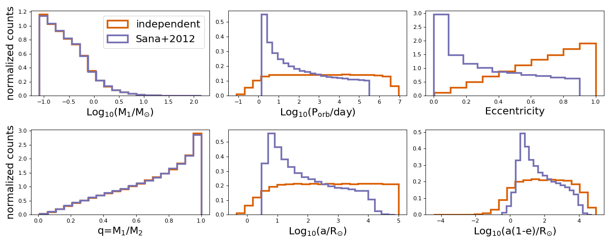
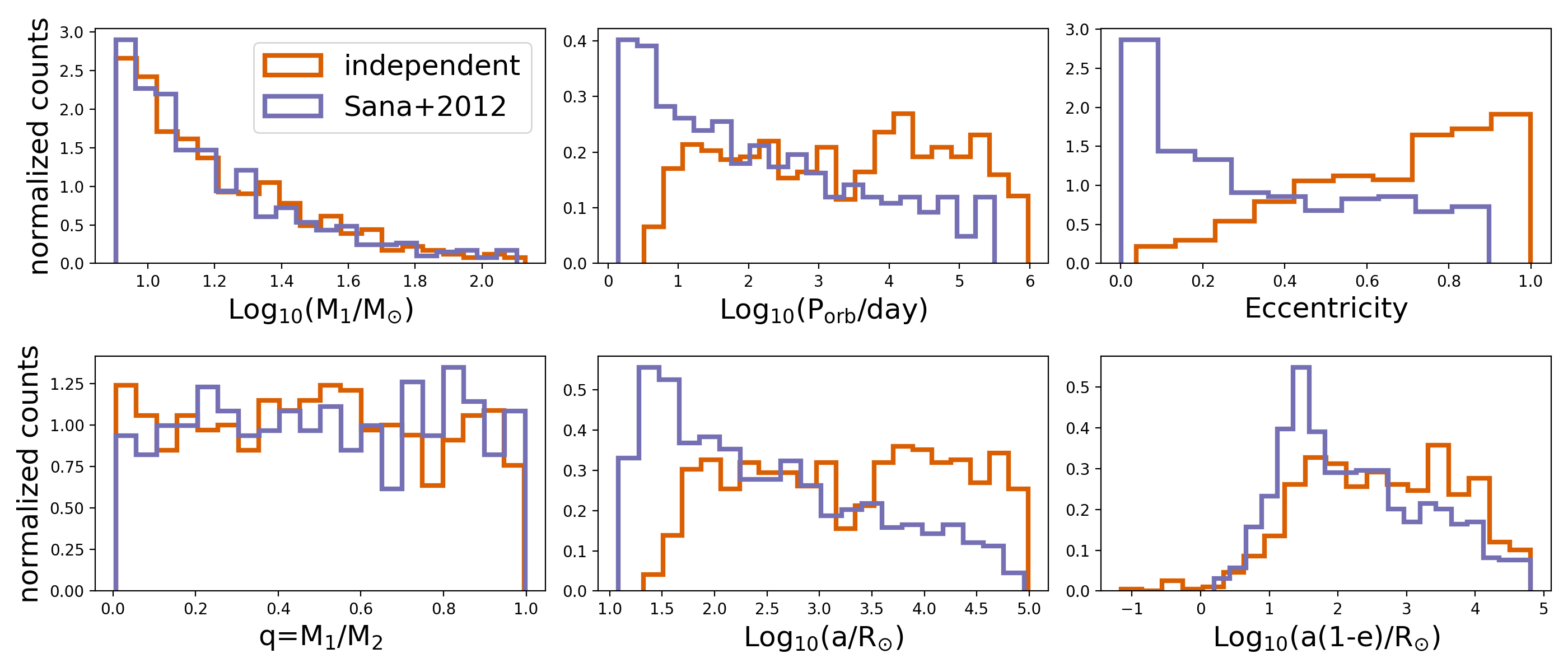
In [7]: InitialBinaries, mass_singles, mass_binaries, n_singles, n_binaries = InitialBinaryTable.sampler('independent', final_kstar1, final_kstar2, binfrac_model=0.5, primary_model='kroupa01', ecc_model='sana12', porb_model='sana12', SF_start=13700.0, SF_duration=0.0, met=0.02, size=10000)

In [8]: print(InitialBinaries)
       kstar_1  kstar_2    mass_1    mass_2          porb       ecc  metallicity   tphysf  ...  epoch_1  epoch_2  tms_1  tms_2  bhspin_1  bhspin_2  tphys  binfrac
0          1.0      1.0  0.877069  0.784652   1052.126265  0.001587         0.02  13700.0  ...      0.0      0.0    0.0    0.0       0.0       0.0    0.0      0.5
1          1.0      0.0  0.843908  0.666603     65.517191  0.017823         0.02  13700.0  ...      0.0      0.0    0.0    0.0       0.0       0.0    0.0      0.5
2          1.0      1.0  1.622439  1.015034      4.732781  0.409041         0.02  13700.0  ...      0.0      0.0    0.0    0.0       0.0       0.0    0.0      0.5
3          1.0      1.0  3.879773  3.778246     35.898711  0.023957         0.02  13700.0  ...      0.0      0.0    0.0    0.0       0.0       0.0    0.0      0.5
4          1.0      1.0  1.552325  0.864780      7.796751  0.218405         0.02  13700.0  ...      0.0      0.0    0.0    0.0       0.0       0.0    0.0      0.5
...        ...      ...       ...       ...           ...       ...          ...      ...  ...      ...      ...    ...    ...       ...       ...    ...      ...
10098      1.0      1.0  9.590471  5.733345  29598.637770  0.194498         0.02  13700.0  ...      0.0      0.0    0.0    0.0       0.0       0.0    0.0      0.5
10099      1.0      1.0  1.569780  0.944479    225.624391  0.404016         0.02  13700.0  ...      0.0      0.0    0.0    0.0       0.0       0.0    0.0      0.5
10100      1.0      1.0  3.058665  2.061208    129.059130  0.064512         0.02  13700.0  ...      0.0      0.0    0.0    0.0       0.0       0.0    0.0      0.5
10101      1.0      1.0  2.722729  2.672297      9.394151  0.413622         0.02  13700.0  ...      0.0      0.0    0.0    0.0       0.0       0.0    0.0      0.5
10102      1.0      1.0  2.925943  2.139549      1.752555  0.042039         0.02  13700.0  ...      0.0      0.0    0.0    0.0       0.0       0.0    0.0      0.5

[10103 rows x 38 columns]
NOTE: the length of the initial binary data set, InitialBinaries, does not always match the size parameter provided to InitialBinaryTable.sampler. This is becuase the sampler accounts for a binary fraction specified by the user with the binfrac_model parameter, which is either a fraction between 0 and 1 or mass dependend following the prescription in van Haaften+2013.
Since we are interested in binaries, we only retain the binary systems that are likely to produce the user specified final kstar types. However, we also keep track of the total mass of the single and binary stars as well as the numbre of binary and single stars so that we can scale our results to larger populations. If you don’t want to filter the binaries, you can supply final kstars as
(Source code, png, hires.png, pdf)

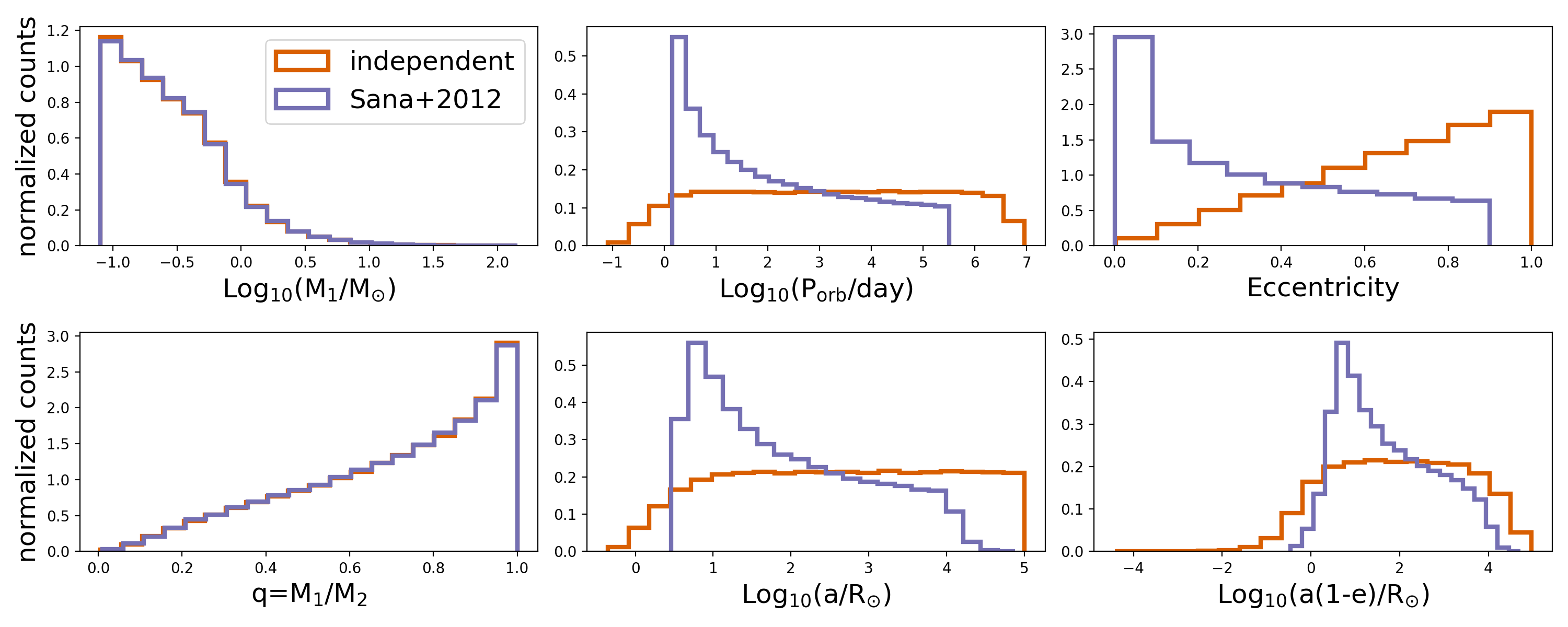
For the entirety of the mass range:  , the mass ratio looks not uniform. This is entirely due to the lower limit of
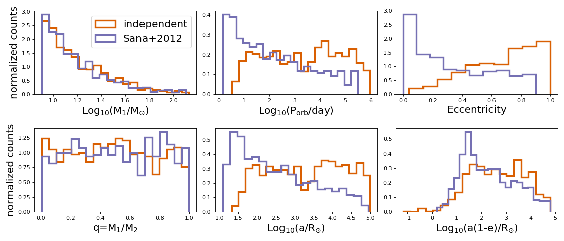
 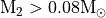 . If we filter on massive stars (
 ), then the mass ratio is totally flat:
(Source code, png, hires.png, pdf)

multidim
COSMIC implements multidimensionally distributed initial binaries according to Moe & Di Stefano 2017. The python code used in COSMIC to create this sample was written by Mads Sorenson, and is based on the IDL codes written to accompany Moe & Di Stefano 2017.
The multidimensional initial binary data is sampled in COSMIC as follows:
In [9]: from cosmic.sample.initialbinarytable import InitialBinaryTable

In [10]: from cosmic.sample.sampler import multidim
To see the arguments necessary to call the multidimensional sampler use the help function:
In [11]: help(multidim.get_multidim_sampler)
Help on function get_multidim_sampler in module cosmic.sample.sampler.multidim:

get_multidim_sampler(final_kstar1, final_kstar2, rand_seed, nproc, SF_start, SF_duration, met, size, **kwargs)
    adapted version of Maxwell Moe's IDL code that generates a population of single and binary stars

    Below is the adapted version of Maxwell Moe's IDL code
    that generates a population of single and binary stars
    based on the paper Mind your P's and Q's
    By Maxwell Moe and Rosanne Di Stefano

    The python code has been adopted by Mads Sørensen

    Version history:
    V. 0.1; 2017/02/03
    By Mads Sørensen
    - This is a pure adaption from IDL to Python.
    - The function idl_tabulate is similar to
    the IDL function int_tabulated except, this function seems to be slightly
    more exact in its solution.
    Therefore, relative to the IDL code, there are small numerical differences.

    Comments below beginning with ; is the original nodes by Maxwell Moe.
    Please read these careful for understanding the script.
    ; NOTE - This version produces only the statistical distributions of
    ;        single stars, binaries, and inner binaries in hierarchical triples.
    ;        Outer tertiaries in hierarchical triples are NOT generated.
    ;        Moreover, given a set of companions, all with period P to
    ;        primary mass M1, this version currently uses an approximation to
    ;        determine the fraction of those companions that are inner binaries
    ;        vs. outer triples. Nevertheless, this approximation reproduces
    ;        the overall multiplicity statistics.
    ; Step 1 - Tabulate probably density functions of periods,
    ;          mass ratios, and eccentricities based on
    ;          analytic fits to corrected binary star populations.
    ; Step 2 - Implement Monte Carlo method to generate stellar
    ;          population from those density functions.

    Parameters
    ----------
    final_kstar1 : `list` or `int`
        Int or list of final kstar1

    final_kstar2 : `list` or `int`
        Int or list of final kstar2

    rand_seed : `int`
        Int to seed random number generator

    nproc : `int`
        Number of processors to use to generate population

    SF_start : `float`
            Time in the past when star formation initiates in Myr

    SF_duration : `float`
            Duration of constant star formation beginning from SF_Start in Myr

    met : `float`
        Sets the metallicity of the binary population where solar metallicity is 0.02

    size : `int`
        Size of the population to sample

    **porb_lo : `float`
        Lower limit in days for the orbital period distribution

    **porb_hi: `float`
        Upper limit in days for the orbital period distribution

    Returns
    -------
    InitialBinaryTable : `pandas.DataFrame`
        DataFrame in the format of the InitialBinaryTable

    mass_singles : `float`
        Total mass in single stars needed to generate population

    mass_binaries : `float`
        Total mass in binaries needed to generate population

    n_singles : `int`
        Number of single stars needed to generate a population

    n_binaries : `int`
        Number of binaries needed to generate a population
The random seed is used to reproduce your initial sample, since there are several stochastic processes involved in the muldimensional sample. As in the independent sampler, the final_kstar1 and final_kstar2 inputs are lists containing the kstar types that the evolved population should contain.
The multidimensional sample is generated as follows:
In [12]: InitialBinaries, mass_singles, mass_binaries, n_singles, n_binaries = InitialBinaryTable.sampler('multidim', final_kstar1=[11], final_kstar2=[11], rand_seed=2, nproc=1, SF_start=13700.0, SF_duration=0.0, met=0.02, size=10)

In [13]: print(InitialBinaries)
   kstar_1  kstar_2     mass_1    mass_2           porb       ecc  metallicity   tphysf  ...  epoch_1  epoch_2  tms_1  tms_2  bhspin_1  bhspin_2  tphys   binfrac
0      1.0      1.0   3.686712  0.806328  161026.959409  0.829034         0.02  13700.0  ...      0.0      0.0    0.0    0.0       0.0       0.0    0.0  0.614692
1      1.0      1.0   0.974390  0.881366      25.334034  0.126290         0.02  13700.0  ...      0.0      0.0    0.0    0.0       0.0       0.0    0.0  0.406506
2      1.0      1.0   2.479799  0.831304      60.621679  0.545004         0.02  13700.0  ...      0.0      0.0    0.0    0.0       0.0       0.0    0.0  0.528636
3      1.0      1.0   1.125074  0.976918   29228.830150  0.713424         0.02  13700.0  ...      0.0      0.0    0.0    0.0       0.0       0.0    0.0  0.411491
4      1.0      1.0   5.805987  3.358740     118.636803  0.718332         0.02  13700.0  ...      0.0      0.0    0.0    0.0       0.0       0.0    0.0  0.795156
5      1.0      1.0  15.916263  6.395108   15884.228362  0.727113         0.02  13700.0  ...      0.0      0.0    0.0    0.0       0.0       0.0    0.0  0.895210
6      1.0      1.0   1.710108  1.069395   55655.129136  0.900815         0.02  13700.0  ...      0.0      0.0    0.0    0.0       0.0       0.0    0.0  0.459633
7      1.0      1.0   2.401816  1.261706     189.173552  0.264586         0.02  13700.0  ...      0.0      0.0    0.0    0.0       0.0       0.0    0.0  0.521047
8      1.0      1.0   2.892138  0.988218     179.329874  0.085426         0.02  13700.0  ...      0.0      0.0    0.0    0.0       0.0       0.0    0.0  0.560256
9      1.0      1.0   2.433570  2.134182   14727.306379  0.261487         0.02  13700.0  ...      0.0      0.0    0.0    0.0       0.0       0.0    0.0  0.521047

[10 rows x 38 columns]
Note
NOTE that in the multidimensional case, the binary fraction is a parameter in the sample. This results in the size of the initial binary data matching the size provided to the sampler. As in the independent sampling case, we keep track of the total sampled mass of singles and binaries as well as the total number of single and binary stars to scale thesimulated population to astrophysical populations.
Evolving an initial binary population
As in Using COSMIC to evolve binaries, once an initial binary population is sampled, it is evolved using the Evolve class. Note that the same process used in Using COSMIC to evolve binaries applies here as well: the BSEDict must be supplied, but only need be resupplied if the flags in the dictionary change.
The syntax for the Evolve class is as follows:
In [14]: from cosmic.evolve import Evolve

In [15]: BSEDict = {'xi': 1.0, 'bhflag': 1, 'neta': 0.5, 'windflag': 3, 'wdflag': 1, 'alpha1': 1.0, 'pts1': 0.001, 'pts3': 0.02, 'pts2': 0.01, 'epsnov': 0.001, 'hewind': 0.5, 'ck': 1000, 'bwind': 0.0, 'lambdaf': 0.5, 'mxns': 2.5, 'beta': 0.125, 'tflag': 1, 'acc2': 1.5, 'remnantflag': 3, 'ceflag': 0, 'eddfac': 1.0, 'ifflag': 0, 'bconst': 3000, 'sigma': 265.0, 'gamma': -1.0, 'pisn': 45.0, 'natal_kick_array' : [[-100.0,-100.0,-100.0,-100.0,0.0], [-100.0,-100.0,-100.0,-100.0,0.0]], 'bhsigmafrac' : 1.0, 'polar_kick_angle' : 90, 'qcrit_array' : [0.0,0.0,0.0,0.0,0.0,0.0,0.0,0.0,0.0,0.0,0.0,0.0,0.0,0.0,0.0,0.0], 'cekickflag' : 2, 'cehestarflag' : 0, 'cemergeflag' : 0, 'ecsn' : 2.5, 'ecsn_mlow' : 1.4, 'aic' : 1, 'ussn' : 0, 'sigmadiv' :-20.0, 'qcflag' : 2, 'eddlimflag' : 0, 'fprimc_array' : [2.0/21.0,2.0/21.0,2.0/21.0,2.0/21.0,2.0/21.0,2.0/21.0,2.0/21.0,2.0/21.0,2.0/21.0,2.0/21.0,2.0/21.0,2.0/21.0,2.0/21.0,2.0/21.0,2.0/21.0,2.0/21.0], 'bhspinflag' : 0, 'bhspinmag' : 0.0, 'rejuv_fac' : 1.0, 'rejuvflag' : 0, 'htpmb' : 1, 'ST_cr' : 1, 'ST_tide' : 0, 'bdecayfac' : 1, 'rembar_massloss' : 0.5, 'kickflag' : 0, 'zsun' : 0.014}

In [16]: bpp, bcm, initC, kick_info  = Evolve.evolve(initialbinarytable=InitialBinaries, BSEDict=BSEDict)

In [17]: print(bcm.iloc[:10])
     tphys  kstar_1   mass0_1    mass_1       lum_1     rad_1        teff_1   massc_1  ...       ecc  B_1  B_2  SN_1  SN_2  bin_state  merger_type  bin_num
0      0.0      1.0  3.686712  3.686712  168.770026  2.337430  13668.603686  0.000000  ...  0.829034  0.0  0.0   0.0   0.0          0         -001        0
0  13700.0     11.0  0.813263  0.813263    0.000003  0.010159   2420.129431  0.813263  ...  0.825647  0.0  0.0   0.0   0.0          0         -001        0
1      0.0      1.0  0.974390  0.974390    0.553692  0.859742   5393.896416  0.000000  ...  0.126290  0.0  0.0   0.0   0.0          0         -001        1
1  13700.0      2.0  0.974245  0.974245    1.834161  1.859697   4947.752034  0.117571  ...  0.126319  0.0  0.0   0.0   0.0          0         -001        1
2      0.0      1.0  2.479799  2.479799   35.960890  1.878811  10358.233251  0.000000  ...  0.545004  0.0  0.0   0.0   0.0          0         -001        2
2  13700.0     11.0  0.626868  0.626868    0.000003  0.012421   2203.269763  0.626868  ... -1.000000  0.0  0.0   0.0   0.0          1         0301        2
3      0.0      1.0  1.125074  1.125074    1.113993  1.028096   5874.533980  0.000000  ...  0.713424  0.0  0.0   0.0   0.0          0         -001        3
3  13700.0     11.0  0.513016  0.513016    0.000057  0.014025   4250.487032  0.513016  ...  0.700281  0.0  0.0   0.0   0.0          0         -001        3
4      0.0      1.0  5.805987  5.805987  892.365648  3.027531  18212.143051  0.000000  ...  0.718332  0.0  0.0   0.0   0.0          0         -001        4
4  13700.0     15.0  0.919179  0.000000    0.019923  0.007311  25474.988978  1.065583  ... -1.000000  0.0  0.0   0.0   0.0          0         -001        4

[10 rows x 39 columns]

In [18]: print(bpp)
           tphys    mass_1    mass_2  kstar_1  kstar_2           sep           porb       ecc  ...  bacc_2  tacc_1  tacc_2     epoch_1       epoch_2  bhspin_1  bhspin_2  bin_num
0       0.000000  3.686712  0.806328      1.0      1.0  20546.178672  161026.959409  0.829034  ...     0.0     0.0     0.0    0.000000  0.000000e+00       0.0       0.0        0
0     227.344776  3.685941  0.806328      2.0      1.0  20549.705506  161082.245996  0.829034  ...     0.0     0.0     0.0   -0.038237  5.418087e-09       0.0       0.0        0
0     228.482113  3.685686  0.806328      3.0      1.0  20550.871772  161100.530537  0.829034  ...     0.0     0.0     0.0   -0.079592  2.001019e-07       0.0       0.0        0
0     229.578244  3.684182  0.806328      4.0      1.0  20557.756119  161208.489095  0.829034  ...     0.0     0.0     0.0   -0.079592  1.427406e-05       0.0       0.0        0
0     274.607762  3.642206  0.806328      5.0      1.0  20751.714592  164264.854622  0.829034  ...     0.0     0.0     0.0   -0.079592  3.164085e-04       0.0       0.0        0
..           ...       ...       ...      ...      ...           ...            ...       ...  ...     ...     ...     ...         ...           ...       ...       ...      ...
9    1016.662854  0.631755  2.309644     11.0      4.0   5482.275639   27430.673325  0.234858  ...     0.0     0.0     0.0  905.359516  1.855961e+02       0.0       0.0        9
9    1228.090578  0.631756  2.278841     11.0      5.0   5540.290247   28014.305982  0.234857  ...     0.0     0.0     0.0  905.359516  1.855961e+02       0.0       0.0        9
9    1232.280357  0.631777  2.247082     11.0      6.0   5600.975843   28632.380178  0.234851  ...     0.0     0.0     0.0  905.359516  1.855961e+02       0.0       0.0        9
9    1233.267203  0.640985  0.608925     11.0     11.0  12583.471598  146330.043967  0.231914  ...     0.0     0.0     0.0  905.359516  1.233267e+03       0.0       0.0        9
9   13700.000000  0.640985  0.608925     11.0     11.0  12583.471599  146330.043981  0.231914  ...     0.0     0.0     0.0  905.359516  1.233267e+03       0.0       0.0        9

[135 rows x 44 columns]