Evolving a single binary
Initial conditions
Below is the process to initialize and evolve a binary that could have formed a GW150914-like binary. First, import the modules in COSMIC that initialize and evolve the binary.
In [1]: from cosmic.sample.initialbinarytable import InitialBinaryTable

In [2]: from cosmic.evolve import Evolve
To initialize a single binary, populate the InitialBinaries method in the InitialBinaryTable class. Each initialized binary requires the following parameters:
m1 : ZAMS mass of the primary star in \(M_{\odot}\)
m2 : ZAMS mass of the secondary star in \(M_{\odot}\)
porb : initial orbital period in days
ecc : initial eccentricity
tphysf : total evolution time of the binary in Myr
kstar1 : initial primary stellar type, following the BSE convention
kstar2 : initial secondary stellar type, following the BSE convention
metallicity : metallicity of the population (e.g. \(Z_{\odot}=0.014\))
In [3]: single_binary = InitialBinaryTable.InitialBinaries(m1=85.543645, m2=84.99784, porb=446.795757,
   ...:                                                 ecc=0.448872, tphysf=13700.0,
   ...:                                                 kstar1=1, kstar2=1, metallicity=0.002)
   ...:

In [4]: print(single_binary)
   kstar_1  kstar_2     mass_1    mass_2  ...  bhspin_1  bhspin_2  tphys  binfrac
0      1.0      1.0  85.543645  84.99784  ...       0.0       0.0    0.0      1.0

[1 rows x 38 columns]
There are two available methods for evaluating the evolution of each star in the binary:
SSE - the single star evolution fitting formulae from Hurley+2000
METISSE - a new stellar evolution package that uses interpolation of detailed stellar models supplied by the user.
You can learn more these choices by consulting the METISSE documentation.
If you have a grid of detailed stellar models and want to use METISSE, you can specify the SSEDict as follows:
In [5]: SSEDict = {'stellar_engine': 'metisse',
   ...:             'path_to_tracks': 'path/to/your/hydrogen/rich/stellar/models/',
   ...:             'path_to_he_tracks': 'path/to/your/helium/stellar/models/'}
   ...:
For now, we will use the default SSE method for evolving single stars in binaries. To do this, we specify the SSEDict which tells COSMIC to use the Hurley fitting formulae.
In [6]: SSEDict = {'stellar_engine': 'sse'}
(Binary) stellar physics assumptions
The flags for the various binary evolution prescriptions used in BSE also need to be set. Each flag is saved in the BSEDict dictionary. Note that the BSEDict only needs to be specified the first time a binary is evolved with COSMIC or if you need to change the binary evolution prescriptions.
If you are unfamiliar with these prescriptions, it is advised to run the defaults from the COSMIC install which are consistent with Breivik+2020, though we don’t promise that these are the most up-to-date prescriptions.
In [7]: BSEDict = {
   ...:     "pts1": 0.001, "pts2": 0.01, "pts3": 0.02, "zsun": 0.014, "windflag": 3,
   ...:     "eddlimflag": 0, "neta": 0.5, "bwind": 0.0, "hewind": 0.5, "beta": 0.125,
   ...:     "xi": 0.5, "acc2": 1.5, "LBV_flag": 1, "alpha1": [1.0, 1.0],
   ...:     "lambdaf": 0.0, "ce2stageflag": 0, "ceflag": 0, "cekickflag": 2,
   ...:     "cemergeflag": 1, "cehestarflag": 0, "qcflag": 5,
   ...:     "qcrit_array": [0.0,0.0,0.0,0.0,0.0,0.0,0.0,0.0,0.0,0.0,0.0,0.0,0.0,0.0,0.0,0.0],
   ...:     "kickflag": 5, "sigma": 265.0, "bhflag": 1, "bhsigmafrac": 1.0,
   ...:     "sigmadiv": -20.0, "ecsn": 2.25, "ecsn_mlow": 1.6, "aic": 1, "ussn": 1,
   ...:     "polar_kick_angle": 90.0,
   ...:     "natal_kick_array": [[-100.0, -100.0, -100.0, -100.0, 0.0], [-100.0, -100.0, -100.0, -100.0, 0.0]],
   ...:     "mm_mu_ns": 400.0, "mm_mu_bh": 200.0, "remnantflag": 4,
   ...:     "fryer_mass_limit": 0, "mxns": 3.0, "fryer_fmix": 1.0,
   ...:     "fryer_mcrit_nsbh": 5.75, "rembar_massloss": 0.5, "wd_mass_lim": 1,
   ...:     "maltsev_mode": 0, "maltsev_fallback": 0.5, "maltsev_pf_prob": 0.1,
   ...:     "pisn": -2, "ppi_co_shift": 0.0, "ppi_extra_ml": 0.0, "bhspinflag": 0,
   ...:     "bhspinmag": 0.0, "grflag": 1, "eddfac": 10, "gamma": -2, "don_lim": -1,
   ...:     "acc_lim": [-1, -1], "smt_periastron_check": 0, "smt_q": -1, "tflag": 1,
   ...:     "ST_tide": 1,
   ...:     "fprimc_array": [2.0/21.0,2.0/21.0,2.0/21.0,2.0/21.0,2.0/21.0,2.0/21.0,2.0/21.0,2.0/21.0,2.0/21.0,2.0/21.0,2.0/21.0,2.0/21.0,2.0/21.0,2.0/21.0,2.0/21.0,2.0/21.0],
   ...:     "ifflag": 1, "wdflag": 1, "epsnov": 0.001, "bdecayfac": 1,
   ...:     "bconst": 3000, "ck": 1000, "rejuv_fac": 1.0, "rejuvflag": 0,
   ...:     "bhms_coll_flag": 0, "htpmb": 1, "ST_cr": 1, "rtmsflag": 0
   ...: }
   ...:
Running a binary
Once the binary is initialized and the BSE model is set, the system is evolved with the the Evolve class, which calls the evolv2.f subroutine in the BSE source code.
In [8]: bpp, bcm, initC, kick_info = Evolve.evolve(initialbinarytable=single_binary, BSEDict=BSEDict, SSEDict=SSEDict)
Output
For every evolved binary system, BSE generates two arrays, which are stored as pandas DataFrames in COSMIC:
bpp - contains binary parameters at important stages in the binary’s evolution, including stellar evolutionary phase changes or mass transfer episodes.
bcm - contains several binary parameters at user specified time steps during the binary’s evolution. The default setting in COSMIC is to output the final stage of the binary at the evolution time specified by the user.
You can see the different parameters included in each DataFrame using the columns attribute of the DataFrame:
In [9]: print(bpp.columns)
Index(['tphys', 'mass_1', 'mass_2', 'kstar_1', 'kstar_2', 'sep', 'porb', 'ecc',
       'RRLO_1', 'RRLO_2', 'evol_type', 'aj_1', 'aj_2', 'tms_1', 'tms_2',
       'massc_he_layer_1', 'massc_he_layer_2', 'massc_co_layer_1',
       'massc_co_layer_2', 'rad_1', 'rad_2', 'mass0_1', 'mass0_2', 'lum_1',
       'lum_2', 'teff_1', 'teff_2', 'radc_1', 'radc_2', 'menv_1', 'menv_2',
       'renv_1', 'renv_2', 'omega_spin_1', 'omega_spin_2', 'B_1', 'B_2',
       'bacc_1', 'bacc_2', 'tacc_1', 'tacc_2', 'epoch_1', 'epoch_2',
       'bhspin_1', 'bhspin_2', 'bin_num'],
      dtype='object')

In [10]: print(bcm.columns)
Index(['tphys', 'kstar_1', 'mass0_1', 'mass_1', 'lum_1', 'rad_1', 'teff_1',
       'massc_he_layer_1', 'massc_co_layer_1', 'radc_1', 'menv_1', 'renv_1',
       'epoch_1', 'omega_spin_1', 'deltam_1', 'RRLO_1', 'kstar_2', 'mass0_2',
       'mass_2', 'lum_2', 'rad_2', 'teff_2', 'massc_he_layer_2',
       'massc_co_layer_2', 'radc_2', 'menv_2', 'renv_2', 'epoch_2',
       'omega_spin_2', 'deltam_2', 'RRLO_2', 'porb', 'sep', 'ecc', 'B_1',
       'B_2', 'SN_1', 'SN_2', 'bin_state', 'merger_type', 'bin_num'],
      dtype='object')
The units are broadly consistent with BSE and are described in Understanding COSMIC outputs.
The evol_type column in bpp indicates the evolutionary change that occurred for each line. The meaning of each number is described here, Evolve Type.
Each of the parameters in bpp or bcm can be accessed in the usual way for DataFrames:
In [11]: print(bpp.mass_1)
0    85.543645
0    78.478571
0    35.306430
0    35.189374
0    35.672987
0    27.963759
0    27.963759
0    27.960385
0    27.460385
0    27.460385
Name: mass_1, dtype: float64

In [12]: print(bpp[['mass_1', 'mass_2', 'kstar_1', 'kstar_2', 'sep', 'evol_type']])
      mass_1     mass_2  kstar_1  kstar_2          sep  evol_type
0  85.543645  84.997840        1        1  1363.435508          1
0  78.478571  78.051230        2        1  1483.589939          2
0  35.306430  81.795246        7        1  1762.728444          2
0  35.189374  81.775263        7        2  1764.789985          2
0  35.672987  37.310862        7        7  2731.073831          2
0  27.963759  28.951666        7        7  3502.090708         16
0  27.963759  28.451666        7       14  3554.204366          2
0  27.960385  28.451666        7       14  3553.625200         15
0  27.460385  28.451666       14       14  3587.991381          2
0  27.460385  28.451666       14       14  3587.192085         10
You can use the utils.convert_kstar_evol_type function to convert the
kstar_1, kstar_2, and evol_type columns from integers to strings
that describe each int:
In [13]: from cosmic.utils import convert_kstar_evol_type

In [14]: convert_kstar_evol_type(bpp)
Out[14]:
          tphys     mass_1     mass_2  ... bhspin_1 bhspin_2  bin_num
0      0.000000  85.543645  84.997840  ...      0.0      0.0        0
0      3.680672  78.478571  78.051230  ...      0.0      0.0        0
0      3.682720  35.306430  81.795246  ...      0.0      0.0        0
0      3.687768  35.189374  81.775263  ...      0.0      0.0        0
0      3.689697  35.672987  37.310862  ...      0.0      0.0        0
0      4.001817  27.963759  28.951666  ...      0.0      0.0        0
0      4.001817  27.963759  28.451666  ...      0.0      0.0        0
0      4.001959  27.960385  28.451666  ...      0.0      0.0        0
0      4.001959  27.460385  28.451666  ...      0.0      0.0        0
0  13700.000000  27.460385  28.451666  ...      0.0      0.0        0

[10 rows x 46 columns]
Note that utils.convert_kstar_evol_type is only applicable to the bpp
array.
Modifying the columns in each table
The columns in each table can be modified by passing in a list of desired columns to the
bpp_columns or bcm_columns keyword arguments in the Evolve.evolve method.
This is useful if you only want a subset of the available columns to reduce memory usage, or if you
want columns from bcm in the bpp table or vice versa.
For example, to only get the time, masses, stellar types, separation, and evolution type, you can do:
In [15]: bpp, bcm, initC, kick_info = Evolve.evolve(
   ....:     initialbinarytable=single_binary,
   ....:     BSEDict=BSEDict,
   ....:     bpp_columns=['tphys', 'mass_1', 'mass_2', 'kstar_1', 'kstar_2', 'sep', 'evol_type']
   ....: )
   ....:

In [16]: print(bpp)
          tphys     mass_1     mass_2  ...          sep  evol_type  bin_num
0      0.000000  85.543645  84.997840  ...  1363.435508          1        0
0      3.680672  78.478571  78.051230  ...  1483.589939          2        0
0      3.682720  35.306430  81.795246  ...  1762.728444          2        0
0      3.687768  35.189374  81.775263  ...  1764.789985          2        0
0      3.689697  35.672987  37.310862  ...  2731.073831          2        0
0      4.001817  27.963759  28.951666  ...  3502.090708         16        0
0      4.001817  27.963759  28.451666  ...  3515.252565          2        0
0      4.001959  27.960385  28.451666  ...  3514.679746         15        0
0      4.001959  27.460385  28.451666  ...  3556.707715          2        0
0  13700.000000  27.460385  28.451666  ...  3555.915388         10        0

[10 rows x 8 columns]
Note
Whichever columns are specified in bpp_columns or bcm_columns, there will always be a bin_num
column included in the output tables to identify each binary uniquely.
Plotting the evolution
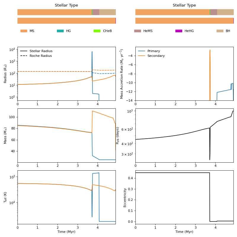
You can also use the built-in plotting function to see how the system evolves:
In [17]: from cosmic.plotting import evolve_and_plot

In [18]: fig = evolve_and_plot(single_binary, t_min=None, t_max=None, BSEDict=BSEDict, SSEDict=SSEDict, sys_obs={})
(Source code, png, hires.png, pdf)
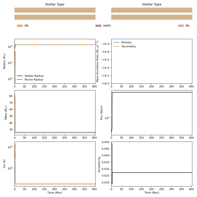
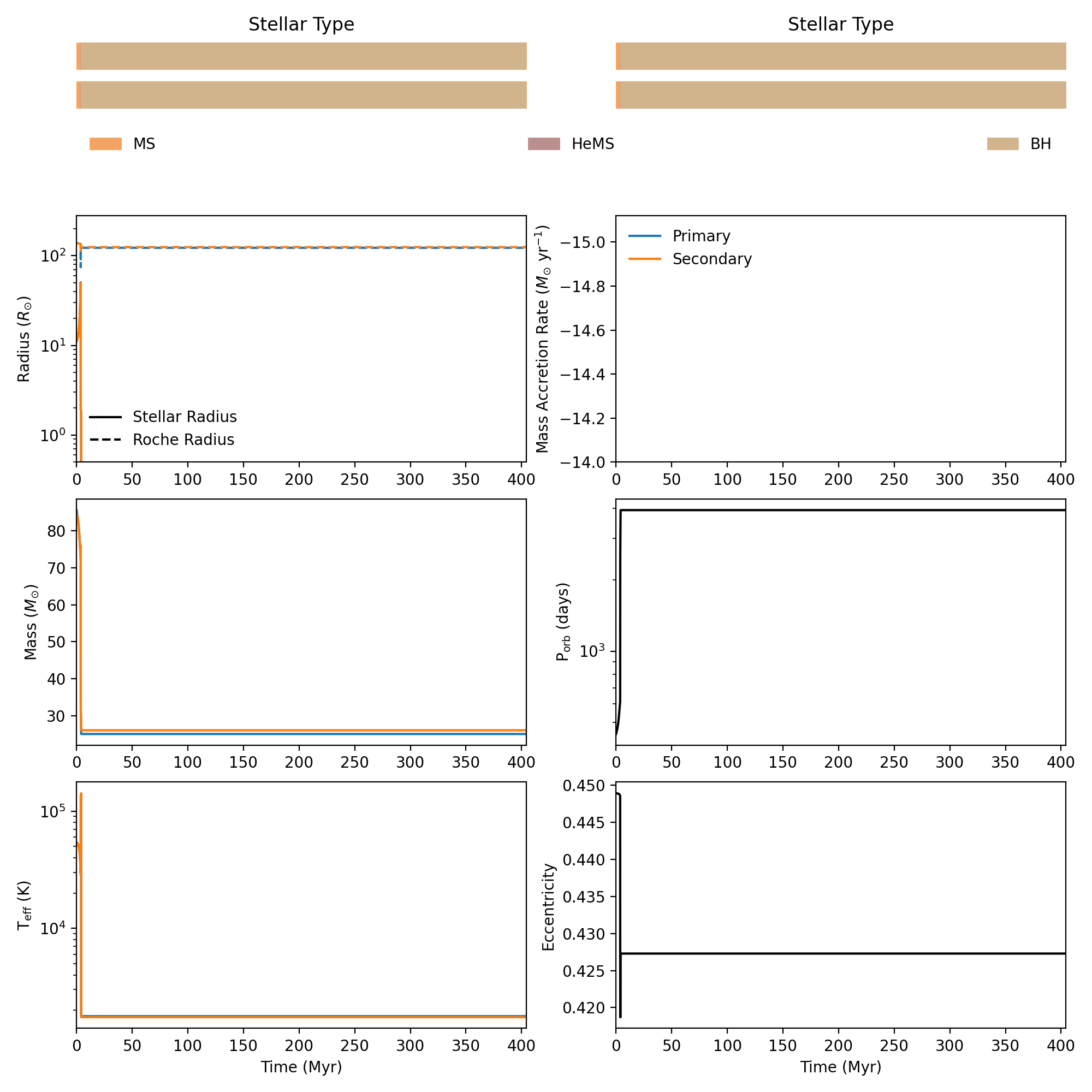
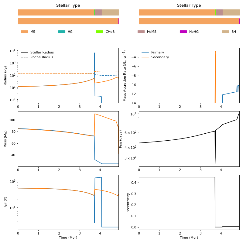
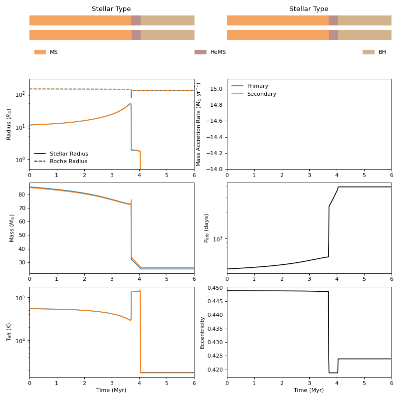
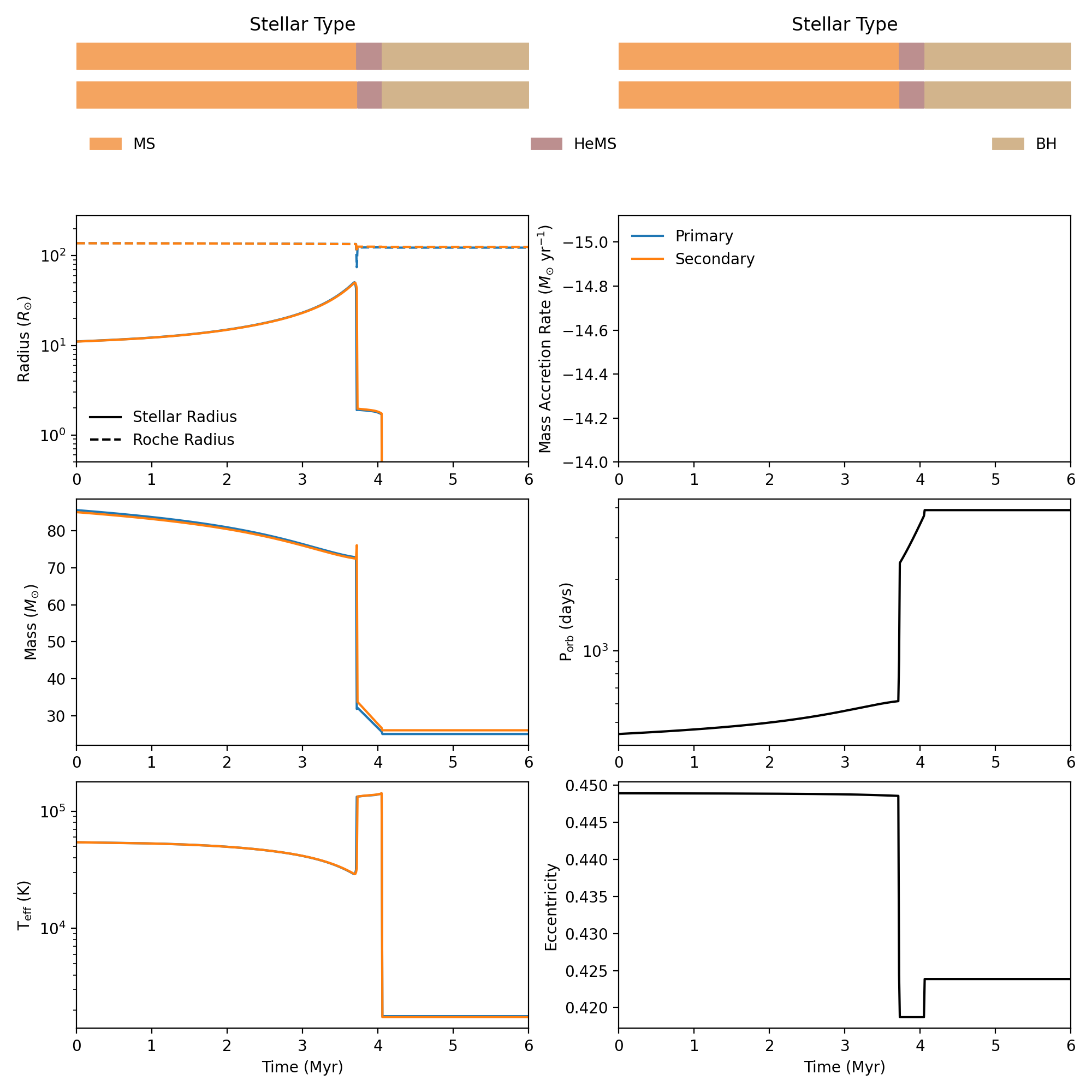
In this case, all the action happens in the first few Myr, so let’s specify a t_max:
In [19]: fig = evolve_and_plot(initC, t_min=None, t_max=6.0, BSEDict=BSEDict, SSEDict=SSEDict, sys_obs={})
(Source code, png, hires.png, pdf)