LBV_flag

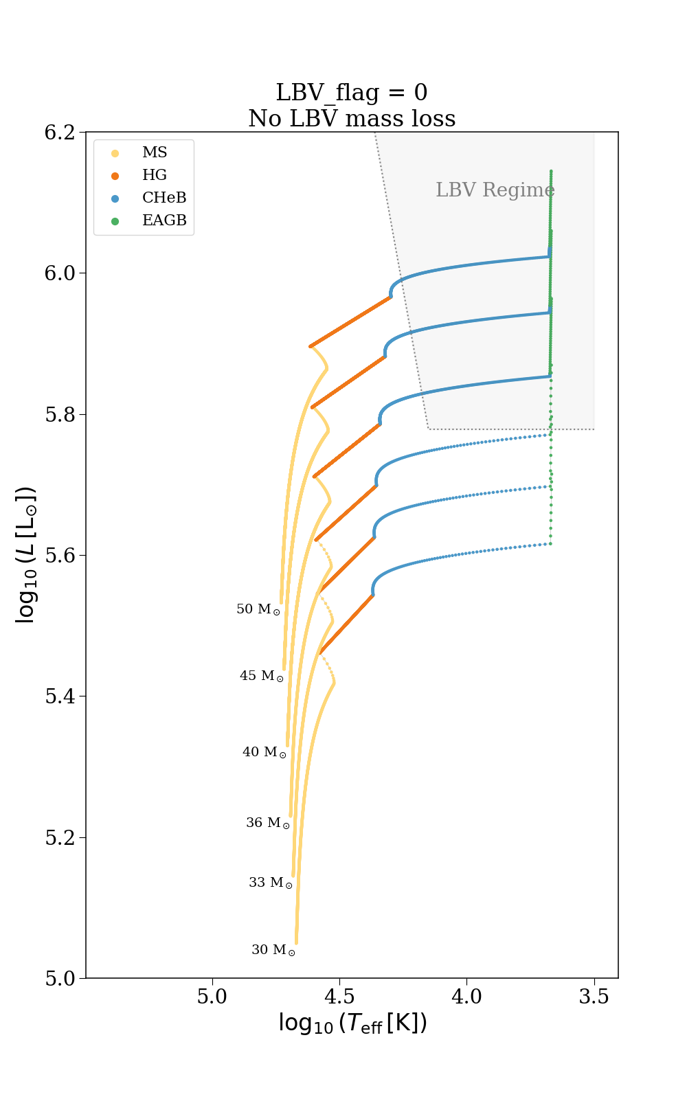
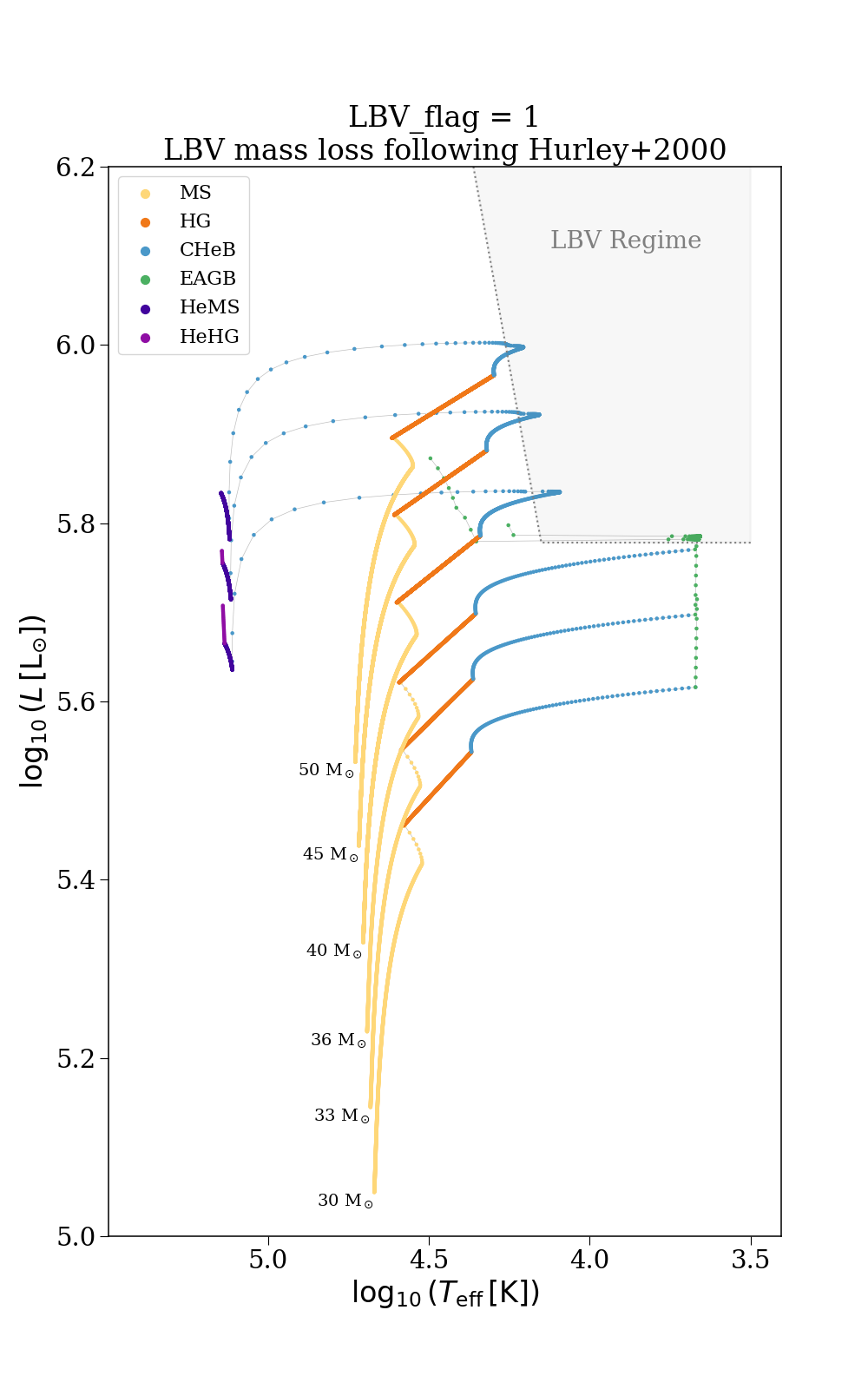
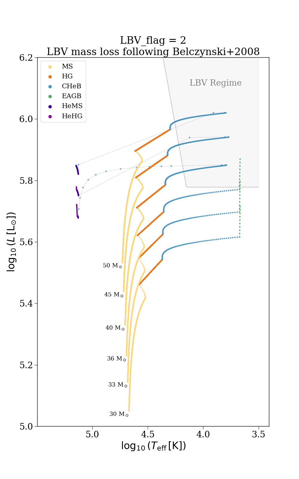
This example shows the effect of the LBV_flag on the evolution of massive stars.

The LBV_flag controls which prescription to use for LBV-like mass loss for stars that are above the Humphreys-Davidson limit. The plots below show the evolution of a few single stars and highlight the LBV regime in which we’d expect to see differences with this flag.

• 
• 
• 

#----------------------------------------------------------------------------------
#----------------------------------------------------------------------------------
## You'll want to edit this part locally to use your own BSEDict and style sheet!

import sys
sys.path.append("..")
import generate_default_bsedict
BSEDict = generate_default_bsedict.get_default_BSE_settings(to_python=True)

import matplotlib.pyplot as plt
plt.style.use("../_static/gallery.mplstyle")
#----------------------------------------------------------------------------------
#----------------------------------------------------------------------------------

import numpy as np
import astropy.units as u
import astropy.constants as consts

from cosmic.sample import InitialBinaryTable
from cosmic.evolve import Evolve
from cosmic.output import kstar_translator

def LBV_limit(T_eff):
    """ Compute the luminosity of the LBV limit given a certain temperature """
    return np.maximum(np.sqrt(1e10 * u.Rsun**2 * u.Lsun * (4 * np.pi * consts.sigma_sb * (T_eff * u.K)**4)).to(u.Lsun), np.repeat(6e5 * u.Lsun, len(T_eff)))


# create a small grid of single stars
masses = [30, 33, 36, 40, 45, 50]
grid = InitialBinaryTable.InitialBinaries(
    m1=masses,
    m2=np.zeros(len(masses)),
    porb=np.ones(len(masses))*-1.0,
    ecc=np.ones(len(masses))*0.0,
    tphysf=np.ones(len(masses))*13700.0,
    kstar1=np.ones(len(masses)),
    kstar2=np.ones(len(masses)),
    metallicity=np.ones(len(masses))*0.014*0.01
)

# loop over different flag choices
for LBV_flag, label in zip([0, 1, 2], ["No LBV mass loss", "LBV mass loss following Hurley+2000",
                                       "LBV mass loss following Belczynski+2008"]):
    # evolve with updated BSEDict
    BSEDict["LBV_flag"] = LBV_flag
    bpp, bcm, initC, kick_info = Evolve.evolve(
        initialbinarytable=grid, BSEDict=BSEDict,
        dtp=0
    )

    # plot a HR diagram of the evolution of these stars, colour coded by kstar
    fig, ax = plt.subplots(figsize=(10, 16))

    for i, bin_num in enumerate(np.unique(bcm["bin_num"])):
        log_teff = np.log10(bcm[bcm["bin_num"] == bin_num]["teff_1"].values)
        log_lum = np.log10(bcm[bcm["bin_num"] == bin_num]["lum_1"].values)
        kstar = bcm[bcm["bin_num"] == bin_num]["kstar_1"].values

        mask = kstar < 10

        ax.scatter(log_teff[mask], log_lum[mask], c=[kstar_translator[k]["colour"] for k in kstar[mask]],
                   s=5)
        ax.plot(log_teff[mask], log_lum[mask], color='grey', alpha=0.5, lw=0.5, zorder=-1)

        # annotate the first point with the initial mass
        ax.annotate(f'{bcm[bcm["bin_num"] == bin_num]["mass_1"].values[0]:.0f} M$_\odot$', (log_teff[0], log_lum[0]),
                    fontsize=14, ha="right", color='black', va='top')

    # annotate the various kstar types
    for k in bcm["kstar_1"].unique():
        if k < 10:
            ax.scatter([], [], color=kstar_translator[k]["colour"], label=kstar_translator[k]["short"], s=50)
    ax.legend()

    # make some fairly reasonable temperature range
    T_eff_range = np.logspace(3.5, 5.4, 1000)

    # plot a line at the HD limit and fill the area
    ax.plot(np.log10(T_eff_range), np.log10(LBV_limit(T_eff_range).value), color="grey", linestyle="dotted")
    ax.fill_between(np.log10(T_eff_range), np.log10(LBV_limit(T_eff_range).value), 9, color="black", lw=2, alpha=0.03)

    # annotate the regime with a custom location
    ax.annotate("LBV Regime", xy=(0.77, 0.93), xycoords="axes fraction", ha="center", va="center",
                fontsize=20, color="grey", zorder=10)

    ax.set(
        xlabel=r"$\log_{10}(T_{\rm eff} \, [\rm K])$",
        ylabel=r"$\log_{10}(L \, [\rm L_{\odot}])$",
        title=f"LBV_flag = {LBV_flag}\n{label}",
        ylim=(5, 6.2)
    )

    ax.invert_xaxis()

    plt.show()