Independent distributions
This guide will show you how to sample an initial binary population using the independent sampler in COSMIC.
First import the InitialBinaryTable class and the independent sampler
In [1]: from cosmic.sample.initialbinarytable import InitialBinaryTable

In [2]: from cosmic.sample.sampler import independent
Tip
The independent sampler contains multiple models for each binary parameter.
You can find the available models here: get_independent_sampler() or by using the independent sampler help call (help(independent.get_independent_sampler))
Targetting specific final kstar types
The final_kstar1 and final_kstar2 parameters are lists that contain the kstar types
that you would like the final population to contain.
The final kstar is the final state of the binary system we are interested in and is based on the BSE kstar naming convention, see Evolutionary State of the Star for more information.
Thus, if you want to generate a population containing double white dwarfs with CO and ONe WD primaries and He-WD secondaries, the final kstar inputs would be:
In [3]: final_kstar1 = [11, 12]

In [4]: final_kstar2 = [10]
Since we are interested in binaries, we only retain the binary systems that are likely to produce the user specified final kstar types. However, we also keep track of the total mass of the single and binary stars as well as the number of binary and single stars so that we can scale our results to larger populations. If you don’t want to filter the binaries, you can supply final kstars as
In [5]: final_kstars = np.linspace(0, 14, 15)

In [6]: InitialBinaries, mass_singles, mass_binaries, n_singles, n_binaries = InitialBinaryTable.sampler(
   ...:     'independent', final_kstars, final_kstars,
   ...:     binfrac_model=0.5, primary_model='kroupa01',
   ...:     ecc_model='sana12', porb_model='sana12',
   ...:     qmin=-1, SF_start=13700.0, SF_duration=0.0,
   ...:     met=0.02, size=10000
   ...: )
   ...:
Additionally if you are interested in single stars then you can specify keep_singles=True. In this case, the singles will be added onto the end of the InitialBinaryTable where kstar_1 will host the singles, kstar_2 will be filled with 15s only, and all orbital properties (e.g. porb or ecc) will be indicated with -1.
Understanding parameter sampling models
Similar to the help for the sampler, the different models that can be used for each parameter to be sampled can be accessed by the help function for the argument. The syntax for each parameter sample is always: sample_`parameter`. See the example for the star formation history (SFH) below:
In [7]: help(independent.Sample.sample_SFH)
Help on function sample_SFH in module cosmic.sample.sampler.independent:

sample_SFH(self, SF_start=13700.0, SF_duration=0.0, met=0.02, size=None)
    Sample an evolution time for each binary based on a user-specified
    time at the start of star formation and the duration of star formation.
    The default is a burst of star formation 13,700 Myr in the past.

    Parameters
    ----------
    SF_start : float
        Time in the past when star formation initiates in Myr
    SF_duration : float
        Duration of constant star formation beginning from SF_Start in Myr
    met : float
        metallicity of the population [Z_sun = 0.02]
        Default: 0.02
    size : int, optional
        number of evolution times to sample
        NOTE: this is set in cosmic-pop call as Nstep

    Returns
    -------
    tphys : array
        array of evolution times of size=size
    metallicity : array
        array of metallicities
Stopping conditions for sampling
In addition to telling COSMIC how to sample, you also need to tell it how much to sample. You can
do this in one of two ways: (1) by specifying the number of binaries to sample, or (2) by specifying the total mass of singles and binaries to sample. Let’s look at both of these in more detail.
Number of binaries
Using the final kstar inputs we mentioned above, the initial binary population can be sampled based on the desired number of binaries (10000 in this case) as follows
In [8]: InitialBinaries, mass_singles, mass_binaries, n_singles, n_binaries = InitialBinaryTable.sampler(
   ...:     'independent', final_kstar1, final_kstar2,
   ...:     binfrac_model=0.5, primary_model='kroupa01',
   ...:     ecc_model='sana12', porb_model='sana12', qmin=-1,
   ...:     SF_start=13700.0, SF_duration=0.0, met=0.02, size=10000
   ...: )
   ...:

In [9]: print(InitialBinaries)
       kstar_1  kstar_2    mass_1    mass_2  ...  bhspin_1  bhspin_2  tphys  binfrac
0          1.0      1.0  3.405783  1.790220  ...       0.0       0.0    0.0      0.5
1          1.0      1.0  1.697957  1.468966  ...       0.0       0.0    0.0      0.5
2          1.0      1.0  1.249914  0.986973  ...       0.0       0.0    0.0      0.5
3          1.0      1.0  5.484669  1.248933  ...       0.0       0.0    0.0      0.5
4          1.0      0.0  1.010395  0.675212  ...       0.0       0.0    0.0      0.5
...        ...      ...       ...       ...  ...       ...       ...    ...      ...
10416      1.0      1.0  0.971809  0.748331  ...       0.0       0.0    0.0      0.5
10417      1.0      1.0  5.056296  2.449137  ...       0.0       0.0    0.0      0.5
10418      1.0      1.0  3.550372  2.863884  ...       0.0       0.0    0.0      0.5
10419      1.0      1.0  1.035552  1.006066  ...       0.0       0.0    0.0      0.5
10420      1.0      1.0  3.780742  1.226972  ...       0.0       0.0    0.0      0.5

[10421 rows x 38 columns]
Note
The length of the initial binary data set, InitialBinaries, does not always match
the size parameter provided to sampler().
This is because of the various cuts that the sampler makes to the population (e.g. the binary fraction,
which is either a fraction between 0 and 1 or mass dependent following the
prescription in van Haaften+2013.) specified by the user.
Total mass sampled
Alternatively, we could do the same thing but now instead set our sampling_target to be the total mass and aim for 15000 solar masses. This is done by setting sampling_target="total_mass" and total_mass=15000.
In [10]: InitialBinaries, mass_singles, mass_binaries, n_singles, n_binaries = InitialBinaryTable.sampler(
   ....:     'independent', final_kstar1, final_kstar2,
   ....:     binfrac_model=0.5, primary_model='kroupa01',
   ....:     ecc_model='sana12', porb_model='sana12',
   ....:     qmin=-1, SF_start=13700.0, SF_duration=0.0,
   ....:     met=0.02,
   ....:     sampling_target="total_mass", total_mass=15000
   ....: )
   ....:

In [11]: print(InitialBinaries)
      kstar_1  kstar_2     mass_1    mass_2  ...  bhspin_1  bhspin_2  tphys  binfrac
0         1.0      1.0   2.409293  1.476737  ...       0.0       0.0    0.0      0.5
1         1.0      1.0   1.088080  0.766619  ...       0.0       0.0    0.0      0.5
2         1.0      1.0   2.303648  0.920767  ...       0.0       0.0    0.0      0.5
3         1.0      1.0   2.128478  0.841482  ...       0.0       0.0    0.0      0.5
4         1.0      1.0   2.548870  1.178500  ...       0.0       0.0    0.0      0.5
...       ...      ...        ...       ...  ...       ...       ...    ...      ...
1342      1.0      1.0   1.094012  0.721110  ...       0.0       0.0    0.0      0.5
1343      1.0      1.0  12.815563  6.323273  ...       0.0       0.0    0.0      0.5
1344      1.0      0.0   0.969117  0.535311  ...       0.0       0.0    0.0      0.5
1345      1.0      1.0  11.990302  2.894143  ...       0.0       0.0    0.0      0.5
1346      1.0      1.0   3.062171  1.817080  ...       0.0       0.0    0.0      0.5

[1347 rows x 38 columns]
And we can check what the total sampled mass was by looking at the sum of the mass_singles and mass_binaries variables
In [12]: print(mass_singles + mass_binaries)
21694.23776613504
Tip
If you’d like to avoid your sample overshooting your desired total_mass and instead get as close to this value as possible,
you can set trim_extra_samples=True. This will trim the sample to get a total mass as close as possible to your target.
In many cases, this will be within a solar mass, but could be as large as twice the maximum stellar mass (for the very rare case that
the final binary drawn is the most massive primary with an equal mass ratio).
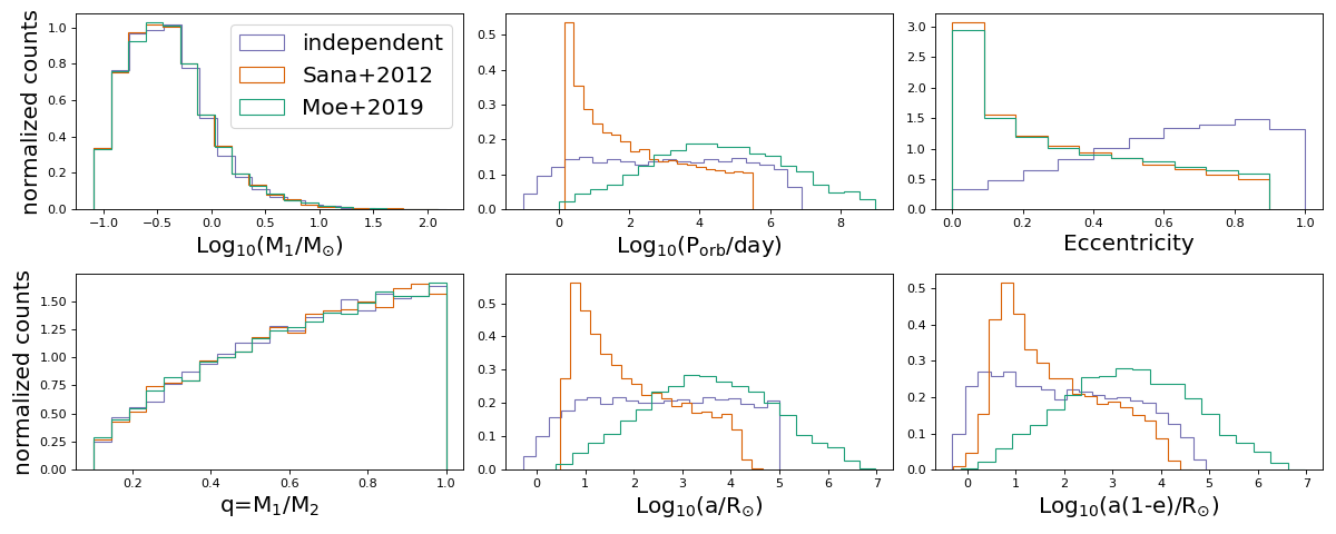
Mass dependent binary fractions and mass pairings
If you want to have separate binary fractions and mass pairings for low and high mass stars, you can by supplying the msort kwarg to the sampler. This sets the mass above which an alternative mass pairing (specified by kwargs qmin_msort and m2_min_msort) and binary fraction model (specified by kwarg binfrac_model_msort) are used. This is handy if you want, for example, a higher binary fraction and more equal mass pairings for high mass stars.
Below we show the effect of different assumptions for the independent initial sampler. The standard assumptions are shown in purple, the assumptions of Sana et al. 2012 are shown in orange, and the assumptions of Moe et al. 2019 are shown in green.
(Source code, png, hires.png, pdf)
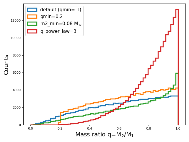
Secondary mass sampling
With the independent sampler, secondary masses are sampled according to a mass ratio model. This model is
defined as a power-law distribution between equal mass systems and a minimum mass ratio, qmin. By default,
the minimum mass ratio is set to -1, which limits the minimum mass ratio to be set such that
the pre-MS lifetime of the secondary is not longer than the full lifetime of the primary if it were to evolve as a single star.
You can change this behavior by setting qmin to a value between 0 and 1.
Alternatively, you can set the minimum mass ratio based off a minimum secondary mass, m2_min. This
is done by setting the m2_min kwarg to a value in solar masses.
In this case, the minimum mass ratio will be calculated as qmin = m2_min / m1, where m1 is the sampled primary mass.
Warning
You cannot set both qmin and m2_min at the same time.
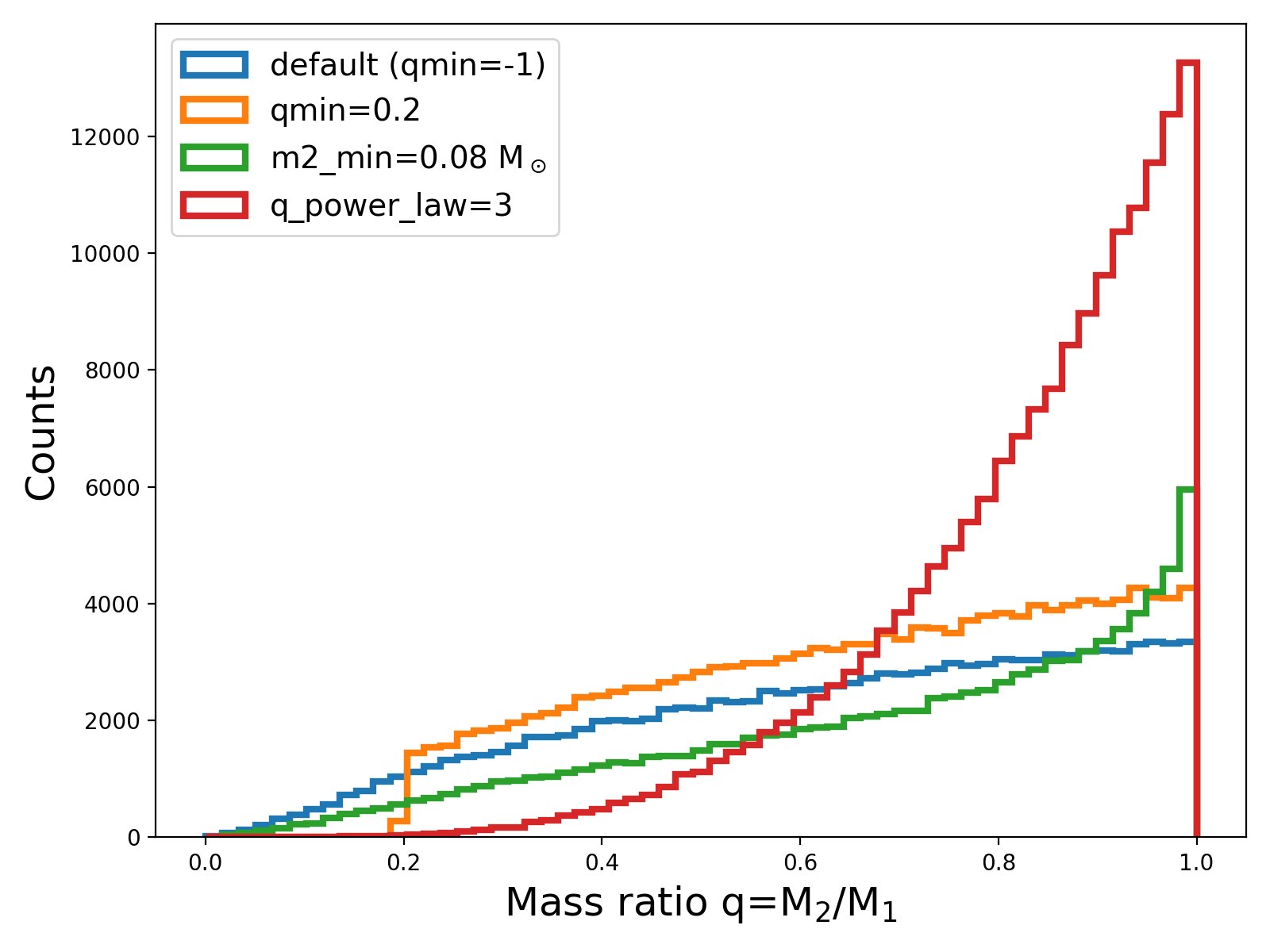
To change the slope of the distribution from which the mass ratio is sampled, you can set the q_power_law kwarg.
By default, this is set to 0, which results in a uniform distribution between qmin and 1.
Let’s try some of this out in practice.
In [13]: common_kwargs = {
   ....:     'final_kstar1' : final_kstars,
   ....:     'final_kstar2' : final_kstars,
   ....:     'binfrac_model' : 1.0,
   ....:     'primary_model' : 'kroupa01',
   ....:     'ecc_model' : 'sana12',
   ....:     'porb_model' : 'sana12',
   ....:     'SF_start' : 13700.0,
   ....:     'SF_duration' : 0.0,
   ....:     'met' : 0.02,
   ....:     'size' : 100000,
   ....:     'trim_extra_samples' : True
   ....: }
   ....:

In [14]: init_bin_qmin = InitialBinaryTable.sampler(
   ....:     'independent',
   ....:     qmin=0.2,
   ....:     **common_kwargs
   ....: )[0]
   ....:

In [15]: init_bin_m2min = InitialBinaryTable.sampler(
   ....:     'independent',
   ....:     m2_min=0.08,
   ....:     **common_kwargs
   ....: )[0]
   ....:

In [16]: init_bin_qpower = InitialBinaryTable.sampler(
   ....:     'independent',
   ....:     q_power_law=3,
   ....:     **common_kwargs
   ....: )[0]
   ....:
Now let’s compare the mass ratio distributions resulting from these different assumptions.
(Source code, png, hires.png, pdf)